EVALUATION DES ERREURS DE CARTES DE VEGETATION AVEC UNE APPROCHE PAR ENSEMBLES FLOUS
Sampling design
Apart from a stratification per eco-geographical area, the sampling design incorporated a two-stage sampling protocol, where aerial photography frames formed the Primary Sampling Units (PSUs). This strategy is employed, for example, by Stehman et al. (03) for the accuracy assessment of the NLCD in the USA. Figures 2.2 to 2.5 display the entire set of PSUs in each of the four study areas. Instead of Landsat pixels as in Stehman et al. (03), a regular 500m-spaced two dimensional grid (thereafter referred as the ‘second stage grid’) formed the set of punctual Secondary Sampling Units (SSUs) of the second stage. Indeed, a scale criterion during map production was to leave out polygons less than 500 meters wide. In order to preserve equal inclusion probabilities at the second stage, the selection of PSUs was done via proportional stratified random sampling as described in Stehman et al. 00 (further discussed via personal communication); this mode of selection was appropriate for including all sparsely distributed classes (a frequent occurrence in our case), in the sample while maintaining a low complexity level of statistics (i.e. standard stratified random formulae). As a compromise between operational costs (our budget for the pilot study) and precision of the estimate, the number of PSUs selected was kept below, though approaching, one fourth of the total number of PSUs in each area. Chapter 2: Accuracy Assessment – 92 – Once the sample PSUs were selected, all points of the second stage grid included within these sample PSUs were assigned to their mapped land cover class. The full second stage sample consisted of 0 points from each class mapped in the area. The selection of this sample was obtained via proportional stratified random sampling from the points contained in the sampled PSUs, this time with a probability inversely proportional to the abundance of the class (see the option of proportional stratified random sampling advocated in Stehman et al.( 00:604). A sequence of ArcView and Excel-based Visual Basic simple routines, for easy and fast repeated use on vector attributes of each class, was specifically designed to perform this proportional selection at both stages.
Verification Design and Analysis
Black and white aerial photography served as the basic material for the reference LULC classifications in all areas under investigation. Their characteristics are described in table 2.3. For instance, the first row indicates that 4 aerial photographs at 1: 37 000 covering the Cuitzeo area and acquired in 99 were used for reference classification via stereoscopic interpretation. The full aerial photographic coverage (2 photographs) acquired in 96 of the Tancítaro volcano and the Uruapan avocado production defined the Tancítaro area. Strong ties between UNAM Geography Institute and local institutions in this relatively small area (the least extended study area of the four) allowed supervised field work to document LULC changes between 96 and 00 that would otherwise have affected our reference data. All air photography at scale 1:75 000 was taken from the INEGI archive. A set of 26 digital ortho-photographs ( from year 00 and from year 96) covered the Tuxtlas area. A 03 photo-interpretation based map at 1: 50 000 from the National Reserves Commission (CONANP) served as the basis for reference classification, especially in areas where the 00 Landsat imagery and 96 ortho-photographs showed contradictory LULC. Finally, 4 aerial photographs from the INEGI archive from January 00 to March 02 covered the Candelaria area and were used for reference classification. One specialist interpreter was assigned to produce reference maplets at a scale of about 1:5 000 on transparent slides for each photographic frame corresponding to a selected Table 2.3. Characteristics of aerial photography used as the main verification dataset for the accuracy assessment of the national forest inventory map. . The reference maplets were drawn according to the community level of classification of the NFI map; a primary and a secondary (alternate) class were assigned to each polygon of the maplet. The allowance for a secondary label was a standard rule to account for the ambiguity of class labelling, either from mixed classes or transitions between classes (ex. ecotones). A confidence rating was applied to photograph interpretation, comparable to the one used in Zhu et al. (00). Wherever the interpreter registered low confidence ratings, his mapping was confirmed or corrected by local information collected in the field. In two areas (Cuitzeo and Candelaria), another specialist (‘local interpreter’) had previously worked on the same material to generate cartography with equal or more precise spatial and taxonomic resolutions. In such cases, any discrepancy in photo-interpretation was turned to the advantage of the ‘local interpreter’. Geometric consistency between the reference material and the NFI map was ensured in a similar way as in Zhu et al. (00): Each sample point (selected SSU) was located on a colour composite of the geo-referenced Landsat image (geometric base of the NFI map) on screen. The location of the point was visually transferred onto the transparent slide over the photographic material. The primary and secondary reference labels of the sample point were then digitally registered according to the photo-interpretation maplet. This step was done by another team member than the specialist photo-interpreter, which added objectivity to the labelling process. Because the SSUs were punctual, we looked for a definition of agreement that would avoid fictitious errors due to the proximity of a polygon edge (and related scale artefacts): We defined agreement between the reference label and the NFI map label when a match occurred between either of the primary or secondary reference labels and any of the NFI map labels within a buffer of 500m of the sample point. This 500m rule was related to scale instructions for map production (see sampling design). A practical inconvenience of the definition was the necessity to manually report NFI map labels which corresponded to the match in the confusion matrix: in case of polygon edge situation, no existing routine permitted us to automatically identify which of the NFI labels within the 500m buffer was the one matching the reference label.
Confusion matrices and global findings
Global accuracy and regional confusion patterns among NFI classes are reported via four confusion matrices (tables 2.4 – 2.7). The same convention as in Stehman et al. (03) was adopted for the matrix format. Indeed, the normalization of matrix elements to total area fractions allows an inter-class confusion pattern analysis per eco-geographical area. Overall agreement scores ranged from 64% (Candelaria) to 78% (Los Tuxtlas). To assist the reader in the ongoing analysis, this interval was used as quantitative bounds of a practical confusion scale: high confusion or low accuracy will thereafter mean accuracy scores lower than 64%, intermediate confusion or accuracy will designate scores between 64 and 78%, and scores above 78% will be labeled as low confusion or high accuracy. As an arbitrary means of separating LULC classes along levels of spatial distribution, we considered three categories of classes: dominant (area fraction above %), common (area Chapter 2: Accuracy Assessment – 97 – fraction between 5 and %), and rare (area fraction below 5%). In order to ease sentences in the analysis, we also introduce the term of ‘confusion flux’ from class a to class b as being the proportion of sampled mapped class a found to belong to class b in the reference data.
Analysis per formation
Accuracy scores were lower in forest-dominated Candelaria (64%) and Tancítaro (67%) areas than in non-forest dominated Cuitzeo (75%) and Los Tuxtlas (78%) areas, possibly because of the higher (confusion-prone) diversity of forest classes than non-forest classes in the NFI classification scheme. For ‘other cover types’ (no vegetation cover, water and human settlement), a high accuracy (79% and above) was registered, with the only exception of the water class in Candelaria, where water bodies are small, dispersed and often seasonal. Visually, the spectral separability of these land covers within the group and with respect to other groups is indeed among the highest on conventionally-used Landsat color composites. The mangrove class also recorded high accuracy in both Candelaria and Los Tuxtlas areas where mangrove is present. Conversely, very high inter-confusion within aquatic nontreed vegetation covers is evident from the matrices when hygrophilous grassland and halophilous vegetation are both present (Cuitzeo and Candelaria). High confusion fluxes also exist from hygrophilous grassland to induced grassland in Los Tuxtlas and Candelaria. The spectral ambiguity and variability (across inundation phases) of these aquatic vegetation types is probably one of the key explainers of this observed high confusion. Former INEGI maps mostly confirm the reference data in exhibiting such errors of the NFI. Trends registered for forest types and land use categories vary according to the eco-geographical area as described below.
Analysis per eco-geographical area Cuitzeo
The global estimate of accuracy in Cuitzeo (figure 2.2) primarily reflects the intermediate score (71%) of the dominant class ‘annual crop’ (table 2.4). The common class oak-pine forest (97%), and rare classes such as sub-tropical scrubland (78%), oak forest (92%), pine Chapter 2: Accuracy Assessment – 98 – forest (79%) and fir forest (76%) record intermediate-high to high accuracy. Therefore, the semi-arid and temperate ‘primary’ vegetation classes present in the area are generally characterized by a low level of confusion. Exceptions are the sole mapped patches of mezquital and cloud forest in Cuitzeo, which both corresponded to other classes on the ground (0% accuracy, double-verified with ground visits). These NFI errors clearly appeared to be omission on respectively reporting change and rectifying an error from INEGI former maps of the area. By contrast with the good agreements obtained for ‘primary’ temperate forest classes, numerous confusions were recorded among classes denominated as temperate forests with secondary vegetation (more exactly with herbaceous, shrub-like and/or secondary vegetation, as stipulated in the NFI classification scheme, which we will label ‘secondary’ forests): According to the reference photo-interpreted data, ‘secondary’ pine forest was wrongly mapped as ‘secondary’ oak, ‘secondary’ mixed (oak-pine) forest was wrongly mapped as ‘secondary’ pine, and oak forest was wrongly mapped as ‘secondary’ mixed forest. These confusions are mainly responsible for the low and very low accuracy levels registered for ‘secondary’ oak (46%), ‘secondary’ pine (%) and ‘secondary’ mixed (45%) forests. Various interpretations may arise from this observation. If we assume that the reference data reflects reality, much area of these ‘secondary’ forests lays on eco-tones even more difficult to discern than for ‘primary’ mixed forests. Indeed, the more pronounced presence of human activity further augments the dimension of class membership to these areas.
GENERAL INTRODUCTION |

