Cours SPSS reading the One-Way Anova Output, tutoriel & guide de travaux pratiques en pdf.
Setting Up the Data
Figure 12.1 presents the variable view of the SPSS data editor where we have defined two variables; one discrete and on continuous. The first variable represents the three different groups that received the three different liquid application treatments. We have given it the variable name group and given it the variable label “Experiment Group.” The second variable represents the number of feathers lost or gained. We have given it the variable name feathers and the variable label “Number of Feathers Lost (-) or Gained (+).”
Since the groups variable represents discrete groups, we need to assign numerical values to each group and provide value labels for each of the groups. Again, this is done by clicking on the cell in the variable row desired (in this case row 1) in the Values column and then clicking on the little gray box that appears, which will open the Value Labels dialogue box. In this dialogue box you can pair numerical values with labels for each of your groups. For this example we have paired 1 with the label “Acid”, 2 with the label “Vinegar”, and 3 with the label “Control Group.”
Running the Analyses
One-Way Anova (See Figure 12.3): From the Analyze (1) pull down menu select Compare Means (2), then select One-Way Anova… (3) from the side menu. In the One-Way Anova dialogue box, enter the variable feathers in the Dependent List: field by left-clicking on the variable and left-clicking on the boxed arrow (4) pointing to the Dependent List: field. Next, enter the variable group in the Factor: field by left-clicking on the variable and left-clicking on the boxed arrow (5) pointing to the Factor: field. Next, request the LSD t-tests by left click the Post Hoc… (6) button.
Figure 12.4 presents the One-Way
Anova: Post Hoc Multiple Comparisons
dialogue box. Here, select the LSD (7) option under the Equal Variances Assumed options. Click Continue (8) to return to the One-Way Anova dialogue box. Next, to request the descriptive statistics for each of the groups and to request a line chart that will plot the group means, left click the Options… button (9; found in Figure 12.3). In the One-Way Anova: Options dialogue box (found in Figure 12.4), select the Descriptive option (10) under Statistics. This will provide you with the sample size, mean, standard deviation, standard error of the mean, and range for each group. Also, select the Means Plot option (11). This will provide you with a line chart that graphs the group means. Left click Continue (12) to return to the One-Way Anova dialogue box. Finally, double check your variables and options and either select OK (13) to run, or Paste to create syntax to run at a later time.
If you selected the paste option from the procedure above, you should have generated the following syntax:
- ONEWAY
- feathers BY group
- /STATISTICS DESCRIPTIVES
- /PLOT MEANS
- /MISSING ANALYSIS
- /POSTHOC = LSD ALPHA(.05).
To run the analyses using the syntax, while in the Syntax Editor, select All from the Run pull-down menu.
Reading the One-Way Anova Output
The One-Way Anova Output is presented in Figures 12.5, 12. 6, and 12.7. This output consists of four major parts: Descriptives (in Figure 12.5), ANOVA (in Figure 12. 5), Multiple Comparison (in Figure 12.6), and the Means Plots (in Figure 12.7).
Reading the Descriptives Output
The descriptives output provides each group’s sample size (N), mean, standard deviation, the standard error of the mean (the standard deviation divided by the square root of N, which estimates the potential for sampling error), and the minimum and maximum scores. Also, this part of the output presents the confidence interval within which we are 95% confident that the true population mean for this group would fall. Like the confidence intervals presented in Chapter 8, this interval is found by adding and subtracting from the mean the 95% confidence limit, which is obtained by multiplying the standard error of the mean by the tcritical associated with n-1 degrees of freedom, at the .05 alpha level. For the most part, we will usually only need to concern ourselves with the means and standard deviations for each of our groups. In this case the means and standard deviations (presented in parentheses) for the acid group, the vinegar group and the control group are -11.00 (3.16228), -2.00(3.12694), and -.5 (2.71825), respectively. Thus, eyeballing our data, we can begin to suspect that the acid group lost significantly more feathers than the other two groups.

