Modeling for Energy Consumption Evaluation
Modeling of Vehicle Propulsion System Vehicle propulsion systems of conventional, battery-electric, and hybrid-electric vehicles are significantly different from each other due to the composition of powertrain components and control system. The main powertrain components are composed of Internal Combustion Engine (ENG), Transmission (TRA), Battery (BAT), and Electric Motor/Generator (EMG), as depicted in Fig.
The main
powertrain components are analytically modeled to estimate the energy consumption of a vehicle over a specified mission in an accurate and rapid way. The analytic models are control-oriented to develop optimal control techniques for hybridelectric vehicles. Moreover, these analytic models are design-oriented as well for the optimization of dimensioning parameters. In other words, they are scalable. As a consequence, the analytic models of powertrain components are established at two Modeling for Energy Consumption Evaluation CHAPTER 2. Modeling for Energy Consumption Evaluation Figure 2.1 – Main powertrain components of a parallel hybrid-electric vehicle. distinct levels: the descriptive and predictive level. At descriptive level, descriptive analytic models describe the main features of a specific powertrain component, such as the energy losses of an ENG. The descriptive analytic model is directly applied for the energy consumption evaluation of any given vehicles, and for the optimal control laws identification for hybrid-electric vehicles. Parameters of descriptive analytic models are identified from each powertrain component. At predictive level, predictive analytic models, on the other hand, allow the prediction of the main features for powertrain components of different dimensioning parameters. For instance, the power losses of an ENG of the varied engine displacements can be approximated by predictive analytic models. Coefficients in predictive analytic models are identified from the identification set of powertrain components in the same family of technology. To validate descriptive and predictive analytic models, estimations are compared with grid-point data. For the sake of clarity, the results estimated by descriptive analytic models alone are designated as description in the following sections; whereas, results approximated by predictive analytic models are designated as prediction. To present the accuracy of descriptive and predictive analytic models, the mean relative error between description and grid point data is denoted by ε d ; whereas, the relative mean error between description and grid-point data is indicated by ε p . Regardless of descriptive or predictive error, the mean relative error, denoted by subscript c, is evaluated for each powertrain component in its identification set. In contrast, the average relative error is evaluated based on the whole identification set, and indicated by the subscript s. Statistic characteristics between estimations (description and prediction) and grid-point data are illustrated to supplement the mean relative error of each component. Apart from the validation at powertrain component and identification set level, the accuracy of descriptive and predictive analytic models is investigated at vehicle propulsion system level. At the propulsion system level, the energy consumption is estimated based on different types of powertrain data for various types of vehicle propulsion systems. The powertrain data consists of grid-point data, description, and prediction; whereas vehicle propulsion systems include conventional, battery-electric, and hybrid-electric vehicles. The accuracy of analytic models is most important at vehicle propulsion system level since it determines their validity. The difference of energy consumption of different vehicle propulsion systems will be demonstrated in Chapter 3.3 and 4.5. Considering the perspective of system identification, the proposed analytic models are needed to validate with components different from the identification set, particularly the predictive analytic models. However, analytic models of powertrain components are validated from the corresponding identification sets due to the availability of data.
Internal Combustion
Engine As the primary power source in a conventional or hybrid-electric vehicle, an internal combustion engine (ENG) provides mechanical power to propel the vehicle by burning hydrocarbon-containing fuels, such as gasoline, diesel, natural gas, and bio-fuels. The ENGs can be classified with respect to various criteria. Concerning the ignition method, there are Spark Ignition (SI) and Compression Ignition (CI) engines. Regarding the charging technology, it is composed of Naturally Aspirated (NA) and Turbo-Charged (TC) method. In regard to NA engines, engineers develop various combustion modes, such as Stoichiometric-Burn (SB) and Lean-Burn (LB) methods.
Dimensioning Parameter
The technological dimensioning parameter of ENGs, denoted by Ie , contains four types of engines for light-duty vehicles, which are combinations of different engine technologies. Four types of engines are listed in Ie = {SI/NA/SB,SI/NA/LB,SI/TC,CI/TC}, and represented by integers in the design optimization of vehicle propulsion systems. Apart from the technological parameter Ie , dimensioning parameters of an engine are essential to develop predictive analytic models. The overall dimensioning parameter set is defined as Se = {Ie ,Ve ,Te ,Pe ,NeT ,NeP }, (2.1) 30 CHAPTER 2. Modeling for Energy Consumption Evaluation where Ve is engine displacement in [m3 ], Te is the rated engine torque in [Nm], Pe is the rated engine power in [kW], NeT and NeP are engine speeds in [rpm] corresponding to the rated torque and the rated power. Although engine displacement, rated torque, and rated power are listed separately, they are not independent from each other. The rated torque and rated power depend on engine displacement because of the similar maximum brake mean effective pressure.
Analytic Model
Parameterization of the engine fuel consumption map is performed for both light- and heavy-duty engines. Accordingly, analytic models at both descriptive and predictive level are developed and validated separately. At Descriptive Level Inspired by the Willans line models [63], the descriptive analytic models of internal combustion engines evaluate the burned fuel power as a function of engine speed and engine brake power. The burned fuel power is converted directly from fuel consumption maps by taking the lower heating value of fuel into account. The chosen descriptive analytic model for light-duty engines is expressed by Pef (ωe ,Pe ) = ke0(ωe ) + ke1(ωe )Pe , Pe ≤ Pec(ωe ) ke0(ωe ) + (ke1(ωe ) − ke2 )Pec(ωe ) + ke2Pe , Pe > Pec(ωe ) , (2.2) where ωe is the engine speed in [rad/s]; Pe is the engine brake power of engine in [W]; Pec is the engine corner power of maximal efficiency [W], whose corresponding torque is depicted in Fig. 2.2; and Pef is the power of burned fuel in [W], which is converted from the mass flow rate of an engine map. Parameters kei(i = 0,1,2) are identified for each individual engine from the engine identification set of Table 2.4. Concerning turbo-charged diesel engines for heavy-duty applications, the descriptive analytic model is Pef (ωe ,Pe ) = ke3(ωe ) + ke4(ωe )Pe + ke5(ωe )P 2 e , (2.3) where parameters kei(i = 3,4,5) are identified for each individual engine in its identification set of Table 2.5. In addition to analytic models of burned fuel power, the full-load torque of an ENG is modeled analytically as well. Concerning SI /N A ENGs for light-duty applications, Engine Figure 2.2 – Corner torque Tec of an internal combustion engine. the analytic model of full-load torque is T e (ωe ) = ke6 + ke7ωe + ke8ω 2 e , (2.4) where T e is the full-load torque. As a convention, variables with over-line (e.g. T ) indicates the maximum admissible value; whereas, the under-line (e.g. T ) represents the minimum admissible value. Parameters kei(i = 6,7,8) are identified by solving the following linear system that contains the engine dimensioning parameters Te , Pe , NeT , and NeP . 1 1000π 30 1000π 30 2 1 NeT π 30 NeT π 30 !2 1 NeP π 30 NeT π 30 !2 ke6 ke7 ke8 = Tek Te 30Pe πNeP , (2.5) where Tek is the engine torque at 1000 rpm for light-duty engines. Regardless of light-duty or heavy-duty engines, turbocharged engines have a piecewise analytic model to approximate the full-load torque, T e (ωe ) = ke9 + ke10ωe , we ≤ πNeT 1 30 Te , πNeT 1 30 ≤ we ≤ πNeT 2 30 ke11 + ke12ωe , we ≥ πNeT 2 30 , (2.6) where NeT 1 and NeT 2 are the minimal and maximal speed of the rated torque, respectively. 32 CHAPTER 2. Modeling for Energy Consumption Evaluation Parameters ke9 and ke10, ke11 and ke12 are identified by solving the following two linear equation systems, 1 1000π 30 1 πNeT 1 30 ke9 ke10 = Tek Te , (2.7) and 1 πNeT 2 30 1 πNeP 30 ke11 ke12 = Te 30Pe πNeP , (2.8) where engine speed NeT 1, NeT 2, and NeP are indicated in Fig. 2.3. Ne [rpm] Te [N m] NeT1 NeT2 Te TeP NeP Figure 2.3 – Speed variables of turbocharged internal combustion engines. At Predictive Level Parameters kei(i = 0,··· ,12) in descriptive analytic models in Eq. 2.2 and 2.3 are further expressed as function of engine dimensioning parameters. As for light-duty engines, their predictive analytic models are expressed by ke0 = Veωe 4π ce1 + 30ce2ωe π , (2.9) ke1 =ce3 + 30ce4ωe π + 900ce5ω2 e π2 , (2.10) ke2 =ce6, (2.11) where coefficients cei(i = 1,··· ,6), depending on engine-technological parameter Ie , are listed in Table 2.1


